Imperfect ground truth: capture-recapture (Common Ground) as the fix
Source:vignettes/callDensity_CommonGround.Rmd
callDensity_CommonGround.RmdTwo-detector test of callDensity R package
Building on the foundation provided by the first vignette, here we attempt to make our simulation even more realistic.
In our first simulation, we simulated a uniform distribution of Antarctic blue whale calls around a hydrophone in a homogenous environment with spherical spreading. We also simulated an automated detector that operated according to a logistic function of SNR. We also simulated false positive detections for the automated detector as an independent normal-distribution in SNR.
We then took a subset of all the calls to simulate annotation of a subset of the data for characterisation of the detectors performance. Specifically, we used the callDensity package to estimate the probability of detecting a single call as a function of SNR from the subset. In our first simulation, we modelled this probabilty of detection using the known ground-truth from the simulation.
In the work of Castro et al. (2024) an expert human observer provides the ground truth annotations. However, not every expert human observers can be “practically perfect in every way,” and some analysts might fall slightly short of that Mary Poppins level of perfection.
In reality, we cannot expect to obtain perfect ground truth data. A more realistic expectation is that we will have detections from more than one observer. Here the term observer includes both algorithms and human observers.
Our goal in this simulation is to explore and understand how imperfect estimation of the ground truth affects our ability to estimate call density.
Again, we start with the density equation:
where: is call density, is number of calls, is false discovery rate, is number of sensors (here always 1), is the duration of data analysed (in hours), is the probability of detection in the study area, and is the study area (in km^2).
Generate known call distribution in space and time.
Start with n calls within radius R of the hydrophone. This should produce a known call density with a uniform random distribution in a circle around the hydrophone. Assuming the recorder is located at centre of study area then distances are the magnitude of the x & y location. A uniform density and increasing area with larger distances should yield a triangular distance distribution.
# 1) Generate a distribution of n calls within radius R of the hydrophone with a
# known call density Uniform random in circle

n = 1e6; # number of simulated calls (regardless of whether detected or not);
R = 1e6; # radius in m (i.e. 1e6=1000km)
k <- 1   # number of sensors (always 1 for single hydrophone moorings)
minDate <- as.POSIXct("2025-01-01")
maxDate <- as.POSIXct("2026-01-01")
Time <- as.numeric(difftime(maxDate,minDate,unit="days"))/(365) # in years

# Call density, D_c is n/A
A = studyArea(R/1e3) # Circular study area in km^2
TrueCallDensity = n/(A*Time) # calls/km^2/time

set.seed(1)
# 1) Generate n uniformly distributed calls within radius R and time period Time
sim <- simCallLocation(n=n, R=R, minDate=minDate, maxDate=maxDate)
cat('Study area (km^2): ', A, '\n')
#> Study area (km^2):  3141593
cat('Number of calls: ', n ,'\n');
#> Number of calls:  1e+06
cat('Time units:', Time, '\n')
#> Time units: 1
cat('True call density (calls per km^2 per unit time): ',TrueCallDensity, '\n')
#> True call density (calls per km^2 per unit time):  0.3183099
Assign sonar equation parameters to each call (SL,NL,TL)
a) Source Level (SL)
Assume source level, SL, is that of Antarctic blue whale song (as in Castro et al. (2024)), a mean of 190 dB re 1 uPa.However, to keep things clearer in this simple example, we use a standard deviation of 4 dB, which is lower than that used by Castro et al. (2024). These values match reasonably well with those that have been estimated for this animal mean of 189 dB and standard deviation of 3-8 dB. Realistic values should help make our simulation better match reality.
b) Noise Level (NL)
We assign NL to each call using a similarly realistic parameters for the distribution of NL.
Our NL distribution resembles the same real-world measurements used by Castro et al. (2024) that were derived from noise samples in the same band, but adjacent in time to the Antarctic blue whale calls they detected. Again, this helps ensure our acoustic environment is somewhat grounded in reality and enhances the plausibility and realism of our simulation.
c) Transmission Loss (TL)
We assign TL to each call using a simple spherical spreading propagation model:
This TL model is a commonly used analytical expression for transmission loss. It is a gross oversimplification compared to real-world transmission losses. However, it has a sound theoretical basis that is readily interpretable (i.e. it’s an inverse square law, which is common in physics).
There has already been some investigations of how uncertainty in TL affects call density (e.g. Helble et al 2013), and TL variability and mismatch is not the focus of this vignette, so there’s reasonable justification for keeping this part simple.
Finally, with our acoustic properties assigned, we apply the passive sonar equation (in dB):
SL <- data.frame(mean=190, sd=4, sampleSize=350) # True SL distribution for sim
NL = data.frame(mean=84, sd = 4, sampleSize = n)  # True NL distribution for sim
tlFunc <- function(r)20*log10(r)

# Simulate the true acoustic properties of each call and false positive
sim <- simCallAcoustics(sim, SL, NL, TL = tlFunc)

# Per-transect estimate of TL (used by callDensity package to estimate pDet)
TL <- simTLradials_20logR(maxRange=R, rangeStep=100, numTransects=4)simCallAcoustics<-
function (sim, SL = data.frame(mean = 190, sd = 4, sampleSize = 350), NL = data.frame(mean = 84, sd = 4, sampleSize = n), TL = function(r) {
    20 * log10(r)
})
{
    n = dim(sim)[1]
    sim$SL <- rnorm(n, mean = SL$mean, sd = SL$sd)
    sim$noiseRMSdB <- rnorm(n, mean = NL$mean, sd = NL$sd)
    sim$TL <- TL(sim$d)
    sim$signalRMSdB <- with(sim, SL - TL)
    sim$snr <- with(sim, SL - TL - noiseRMSdB)
    return(sim)
}
simTLradials_20logR <-
function (maxRange, rangeStep, numTransects)
{
    range_m = seq(from = 5, to = maxRange, by = rangeStep)
    tlTransectSpherical <- 20 * log10(range_m)
    tlTransects <- replicate(numTransects, tlTransectSpherical)
    angleStep <- 360/numTransects
    angles = seq(from = 0, to = 360 - angleStep, by = angleStep)
    colnames(tlTransects) <- paste0("tl", angles)
    TL <- data.frame(range_m)
    TL <- cbind(TL, tlTransects)
    return(TL)
}
Simulate detection process
To simulate the detection process we need to make some assumptions about the behaviour of the detector.
Generally, if not by definition, a detector has a higher probability of detection at high SNR, and a lower probability of detection at low SNR. In quantitative sonar performance modelling sometimes a step-function or logistic curve is used when an analytical expression is required. If ground truth data on the detectors performance are available, these models can be fit to the detection data.
Assume probability of detection, p_det, for both detectors follows a logistic curve with SNR as the only independent variable. We can assign a location/intercept for this curve (i.e. location along x-axis where p_det=0.5). We can also assign a scale/slope of the curve to represent the steepness of the transition between low proability and high probability.
Simulate false positives
In addition to the probability of detection, there is also a probability of false alarm (false positive predictions) that we would like to simulate as well.
There can be multiple mechanisms that can produce false positives. For example, they could be triggered by intense high-SNR sound in the same band as the signal, but from a different source. For some signal types, false positives can also arise from small deviations in ambient noise (producing false positive detections that contain very low SNR). Again, if ground truth data are available then the relationship between false positive detections and false-positive power to noise ratio (SNR of false positives) can be modeled in a similar manner to that of probability of detection.
Here we assume false positive detections are distributed around some mean low SNR. This means that false positives in the ‘ground truth’ detector can affect the pDet~SNR curve/function.
Parameterise detectors
Summary of detectors:
| Detector | Description | Location/SNR ‘threshold’ | Scale/slope | False positive rate |
|---|---|---|---|---|
| Detector 1 | Reliable and good detector, meant to emulate a human analyst. | Lower | Same | Lower |
| Detector 2 | Automated detector, meant to emulate a signal processing algorithm. | Higher | Same | Higher |
#Specify parameters for detector 1
# Good detector with low threshold (location) and low false positive rate.
det1params = data.frame(
  location=1,    # AKA intercept?
  scale=2,       # AKA slope?
  func='plogis', # logistic function
  c=0.1,         # False discovery rate
  fpMean=0,      # Mean of distribution of false positives (in dB SNR)
  fpSD = 2      # Standard deviation false positive distribution (in dB SNR)
)

# Detector 2 has a higher threshold (location), scale, and false positive rate
# than detector 1.
det2params = data.frame(
  location=2,    # AKA intercept?
  scale=4,       # AKA slope?
  func='plogis', # logistic function
  c=0.3,         # False discovery rate
  fpMean=0,      # Mean of distribution of false positives (in dB SNR)
  fpSD = 2      # Standard deviation false positive distribution (in dB SNR)
)
Now we create a function that will take the detector parameters above and simulate the detection process. We then call this function with each set of parameters to create a simulation for each detector.
# Simulate two detectors each with the different parameters
simDet1<- simulateDetector(det1params,sim)
simDet2<- simulateDetector(det2params,sim)simulateDetector <-
function (detParams, sim)
{
    sim$p_det = plogis(sim$snr, location = detParams$location, scale = detParams$scale)
    sim$detect_table <- as.logical(rbinom(dim(sim)[1], size = 1, prob = sim$p_det))
    n_tp <- sum(sim$detect_table)
    n_fp <- as.integer(n_tp/(1 - detParams$c) - n_tp)
    if (n_fp > 0) {
        fp <- data.frame(matrix(ncol = length(sim), nrow = n_fp))
        colnames(fp) <- colnames(sim)
        fp$groundTruth <- FALSE
        fp$detect_table <- TRUE
        duration_s <- as.numeric(difftime(max(sim$datetime), min(sim$datetime), units = "sec"))
        fp$datetime <- uniqueEventTimes(n_fp, min(sim$datetime), duration_s, avoid = sim$datetime)
        fp$noiseRMSdB <- rnorm(n_fp, mean = mean(sim$noiseRMSdB, na.rm = TRUE), sd = sd(sim$noiseRMSdB, na.rm = TRUE))
        fp$snr <- rnorm(n_fp, mean = detParams$fpMean, sd = detParams$fpSD)
        fp$signalRMSdB <- fp$noiseRMSdB + fp$snr
        sim <- rbind(sim, fp)
    }
    sim$group <- factor(ifelse(sim$groundTruth, ifelse(sim$detect_table, "TruePositive", "FalseNegative"), "FalsePositive"), levels = c("FalsePositive", "TruePositive", "FalseNegative"))
    return(sim)
}
View the spatial detection density (which is not the same as spatial call density since it accounts for neither detection probability nor time).
sp1 <- plotSpatialDetections(simDet1)+ggtitle('Detector 1')
sp2 <- plotSpatialDetections(simDet2)+ggtitle('Detector 2')
gridExtra::grid.arrange(sp1,sp2,nrow=1)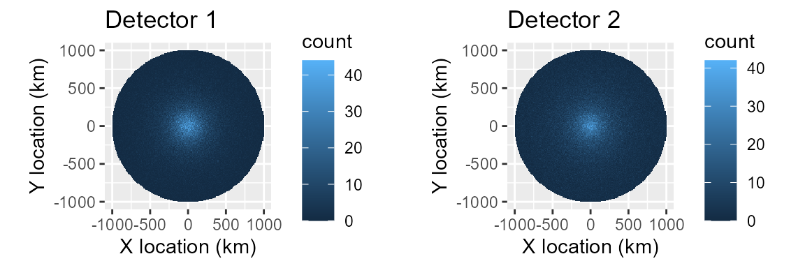
dist1 <- plotDetectionDistribution(simDet1)+ggtitle('Detector 1')
dist2 <- plotDetectionDistribution(simDet2)+ggtitle('Detector 2')
gridExtra::grid.arrange(dist1,dist2,nrow=1)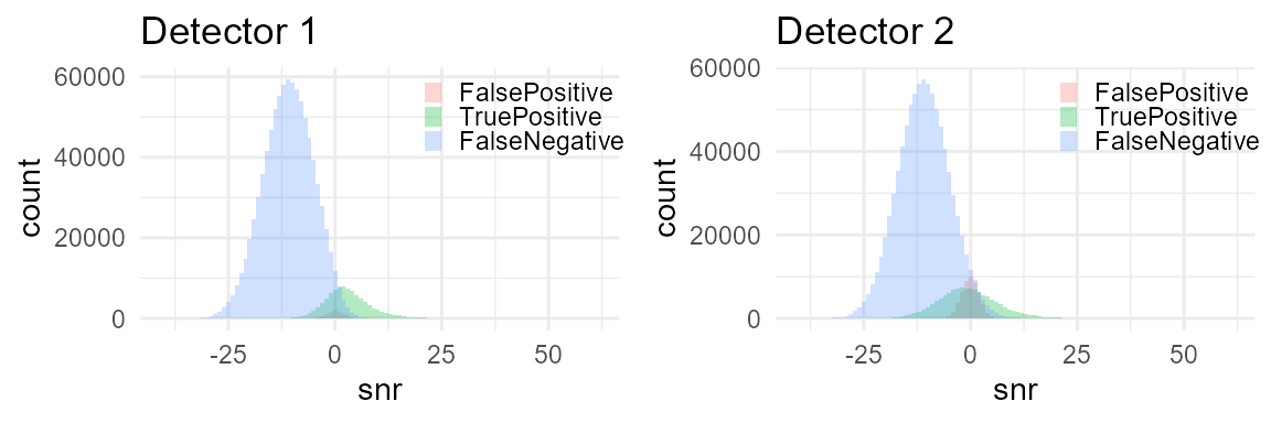
Subsample data for detector characterisation
Castro et al. (2024) subsample approximately 200 hours evenly spaced throughout the year to create detector characterisation curves (detection vs SNR). Here we subsample 1 hour in every 41 hours yielding 214 subsamples that are 1 hour in duration.
subsampleDet1 <- subsampleSimInTime(simDet1,interval = "41 hour")
subsampleDet2 <- subsampleSimInTime(simDet2,interval = "41 hour")subsampleSimInTime <-
function (cht, minDate = NULL, maxDate = NULL, interval = "41 hour", duration = 3600, timeCol = "t0")
{
    if (!timeCol %in% names(cht)) {
        if (timeCol == "t0" && "datetime" %in% names(cht)) {
            timeCol <- "datetime"
        }
        else {
            stop("subsampleSimInTime: no column named '", timeCol, "' in the input.", call. = FALSE)
        }
    }
    tvals <- cht[[timeCol]]
    if (!inherits(tvals, "POSIXct"))
        tvals <- mat2Rdate(tvals)
    if (any(is.na(tvals))) {
        stop("subsampleSimInTime: column '", timeCol, "' contains ", sum(is.na(tvals)), " NA value(s); cannot window on it.", call. = FALSE)
    }
    if (is.null(minDate))
        minDate <- min(tvals)
    if (is.null(maxDate))
        maxDate <- max(tvals)
    subStart <- seq(from = minDate, to = maxDate, by = interval)
    subEnd <- subStart + duration
    keep <- rep(FALSE, length(tvals))
    for (i in seq_along(subStart)) {
        keep <- keep | (tvals >= subStart[i] & tvals <= subEnd[i])
    }
    out <- cht[keep, , drop = FALSE]
    rownames(out) <- NULL
    out
}
ggplot(subsampleDet1, aes(x=datetime, weights=detect_table) )+
  # geom_point(size=1,alpha=0.1)
  geom_histogram(breaks=seq(from=minDate,to=maxDate,by='12 h'))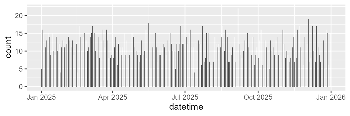
ggplot(subsampleDet2, aes(x=datetime, weights=detect_table) )+
  # geom_point(size=1,alpha=0.1)
  geom_histogram(breaks=seq(from=minDate,to=maxDate,by='12 h'))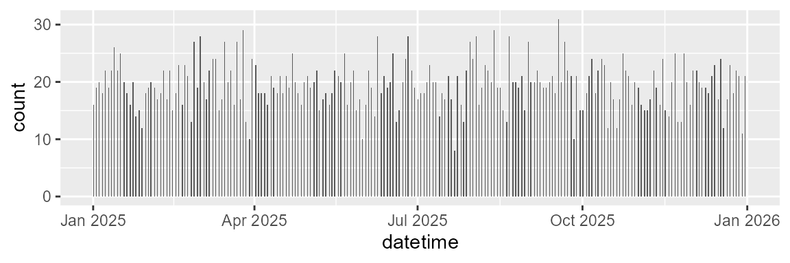
Detection matching between detector 1 and 2
Both detectors (simulated subsets) operate on the same set of calls (i.e. they are different subsets of the same underlying simulation). So we can find detections from one detector that match those of the other detector by merging the detections into a capture history table. We accoomplish this with by a full-outer join of the tables with the timestamp/datetime, as the key/matching-variable.
NB: Real world detections from independent observers rarely have timestamps that match exactly, so real data would require matching criteria that can accomodate some amount of error in detection times, locations, and other parameters.
Presently, false positives have randomly generated date-times, so have a negligible chance of matching between the two detectors (i.e. false positives on one detector are independent from the other). In reality false-positives are unlikely to be fully independent, so there is an opportunity to improve the realism of the simulation by estimating correlation in false positives for real datasets, and then simulating that relationship here.
TODO: Create false positives in a way that better approximates their real-world occurrence (i.e. in a way that allows them to be matched between detectors).
capHistTab <- simsTocaptureHistoryTable(subsampleDet1, subsampleDet2)

# simsTocaptureHistoryTable() keeps every observer's own signal/noise/SNR
# columns separately, suffixed (matchbox-native), rather than
# auto-consolidating them the way it used to. cde()'s own
# falseDiscoveryRate() call needs a single SNR column for its truncation
# handling (a separate mechanism from chtToSNRinfo()'s signalCol/noiseCol
# averaging below), so that's built explicitly here.
capHistTab$SNR <- rowMeans(capHistTab[, c("snr_observer1", "snr_observer2")], na.rm = TRUE)simsTocaptureHistoryTable <-
function (..., observerSuffix = NULL)
{
    detectors <- list(...)
    n <- length(detectors)
    if (n < 2) {
        stop("simsTocaptureHistoryTable: need at least two detectors.", call. = FALSE)
    }
    if (is.null(observerSuffix)) {
        observerSuffix <- paste0("observer", seq_len(n))
    }
    if (length(observerSuffix) != n) {
        stop("simsTocaptureHistoryTable: observerSuffix must have one entry per ", "detector (", n, " detectors, ", length(observerSuffix), " suffixes given).", call. = FALSE)
    }
    dupCounts <- vapply(detectors, function(d) sum(duplicated(d$datetime)), integer(1))
    if (any(dupCounts > 0)) {
        stop("simsTocaptureHistoryTable: detector(s) ", paste(which(dupCounts > 0), collapse = ", "), " contain duplicated datetime values (", paste(dupCounts[dupCounts > 0], collapse = ", "), " duplicate(s) respectively). Merging on a duplicated key produces ", "a cartesian product: k duplicates shared across ", n, " detectors give k^", n, " rows for one event. Every event must ", "have a unique datetime. See uniqueEventTimes().", call. = FALSE)
    }
    suffixed <- lapply(seq_len(n), function(i) {
        d <- detectors[[i]]
        isKey <- names(d) == "datetime"
        names(d)[!isKey] <- paste0(names(d)[!isKey], "_", observerSuffix[i])
        d
    })
    cht <- Reduce(function(a, b) merge(a, b, by = "datetime", all = TRUE), suffixed)
    for (i in seq_len(n)) {
        rawDetectCol <- paste0("detect_table_", observerSuffix[i])
        newDetectCol <- paste0("detect_", observerSuffix[i])
        names(cht)[names(cht) == rawDetectCol] <- newDetectCol
        cht[[newDetectCol]][is.na(cht[[newDetectCol]])] <- FALSE
        cht[[newDetectCol]] <- as.logical(cht[[newDetectCol]])
    }
    gtCols <- paste0("groundTruth_", observerSuffix)
    if (all(gtCols %in% names(cht))) {
        cht$groundTruth <- as.logical(Reduce(function(a, b) ifelse(is.na(a), b, a), cht[gtCols]))
    }
    cht <- cht[order(cht$datetime), ]
    cht$key <- seq_len(nrow(cht))
    cht$t0 <- Rdate2mat(cht$datetime)
    cht$tEnd <- Rdate2mat(cht$datetime)
    rownames(cht) <- NULL
    cht
}
Convert this capture history table into an SNRinfo table, and treat detector1 as ground truth.
# SNRinfo is used to calculate snrDetFun for detector2 assuming detector1 is the
# ground truth. This is an observer ground (OG) so includes false positives from
# detector1, but does not include detections from detector2 not detected on
# detector1. signalCol/noiseCol point at each observer's own suffixed
# signal/noise columns, which chtToSNRinfo() averages per event -- there is
# no single consolidated signalRMSdB/noiseRMSdB column to fall back on.
SNRinfo <- chtToSNRinfo(capHistTab, groundTruth = "observer1", observers = "observer2",
                        signalCol = c("signalRMSdB_observer1", "signalRMSdB_observer2"),
                        noiseCol  = c("noiseRMSdB_observer1",  "noiseRMSdB_observer2"))

# Positive on detector 2, but not on 1
n_fp_subsample <- sum(capHistTab$detect_observer2 & !capHistTab$detect_observer1)
n_p_subsampleDet2 <- sum(capHistTab$detect_observer2)

# False discovery rate is number.false.positives/number.predicted.positive
c_subsample <- n_fp_subsample/n_p_subsampleDet2
n_subsample <- dim(SNRinfo)[1]  # Number positive detections in SUBset

truncationDistances <- R

# Number positive detections in FULL set
Nc <- sum(simDet2$detect_table)

# Noise level from subsampled Observer ground-truth
NLsamp <- SNRinfo %>% dplyr::summarise(mean=mean(NoiseRL,na.rm = TRUE),
                             sd=sd(NoiseRL,na.rm = TRUE),
                             sampleSize=dplyr::n()-sum(is.na(NoiseRL)))

NLtable <- rbind(NL,NLsamp)
rownames(NLtable)<- c('Actual','Estimated from subsample')
kable(NLtable,caption = 'Noise level distributions')%>%
kableExtra::kable_classic(full_width=FALSE)| mean | sd | sampleSize | |
|---|---|---|---|
| Actual | 84.00000 | 4.000000 | 1000000 |
| Estimated from subsample | 81.16079 | 3.941931 | 2389 |
Calculate call densities using callDensity package
GLM fit to SNR detection function
The detector was a logistic function, so fitting a GLM should provide good results.
A GAM or SCAM should also be able to provide a good fit to a logistic function, but to keep this concise we leave fitting those as an exercise for the reader (see callDensity vignette).
The callDensity package provides a convenience function fitDetFun to fit GLM, GAM, and SCAM models:fitDetFun <-
function (SNRinfo, modelType = c("gam", "glm", "scam", "vglm"), numKnots = 3, yColNames = c("detect_observer1", "detect_observer2"), whichObserver = NULL)
{
    modelType <- match.arg(modelType)
    res <- switch(modelType, glm = stats::glm(Detected ~ SNR, data = SNRinfo, family = stats::binomial()), gam = mgcv::gam(Detected ~ s(SNR, k = numKnots), data = SNRinfo, family = stats::binomial()), scam = scam::scam(Detected ~ s(SNR, k = numKnots, bs = "mpi"), data = SNRinfo, family = stats::binomial()), vglm = {
        fit <- VGAM::vglm(as.matrix(SNRinfo[, yColNames]) ~ SNR, VGAM::posbernoulli.t(parallel.t = TRUE ~ 0), data = SNRinfo)
        if (is.null(whichObserver)) whichObserver <- tail(yColNames, 1)
        fit@extra$whichObserver <- whichObserver
        fit@extra$yColNames <- yColNames
        fit
    })
    attr(res, "modelType") <- modelType
    if (!isS4(res)) {
        class(res) <- c("detFun", class(res))
    }
    res
}
snrDetFun.glm <- callDensity::fitDetFun(SNRinfo, modelType = "glm")

results.glm <- cde(Nc=Nc, capHistTab = capHistTab, snrDetFun = snrDetFun.glm,
                   SL = SL, TL = TL, NL=NLsamp, A = A, modelType = 'glm',
                   groundTruthCol = "detect_observer1", observerCol = "detect_observer2",
                   signalCol = c("signalRMSdB_observer1", "signalRMSdB_observer2"),
                   noiseCol  = c("noiseRMSdB_observer1",  "noiseRMSdB_observer2"))
Results
Table showing how the the results of the estimated call density compare to the true values.
results.true = data.frame(season='year',    siteCode='',  Nc=n, c=det2params$c,
                          k=1, T=Time, A=A, pa=mean(simDet2$p_det,na.rm=TRUE),
                          SLmean=SL$mean, SLsd=SL$sd, NLmean=NL$mean, NLsd=NL$sd,
                          modelType='true', CV.Nc=0, CV.c=0, CV.pa=0,
                          Dc=TrueCallDensity,  CV.Dc=0)

results<-rbind( results.true, results.glm)
res <- subset(results,select=c('Dc','Nc','A','NLmean','NLsd','modelType','c',
                               'pa') )
kableExtra::kbl(res, digits = c(4,3,0,1, 2, NA, 3, 4),
                col.names= c('Dc','(sub)Sample Size', 'A','NL_mean','NL_sd',
                             'Model','c','P_a')) %>%
kableExtra::kable_classic(full_width=FALSE)| Dc | (sub)Sample Size | A | NL_mean | NL_sd | Model | c | P_a |
|---|---|---|---|---|---|---|---|
| 0.3183 | 1000000 | 3141593 | 84.0 | 4.00 | true | 0.300 | 0.1208 |
| 0.0981 | 173205 | 3141593 | 81.2 | 3.94 | glm | 0.722 | 0.1563 |
In this scenario, our estimate of Dc is far from the true value.
It appears that the estimates of mean noise level are all lower than the actual value. Using the lower mean for the NL distribution yields a higher value for P_a, which creates a bias in the estimate of Dc.
This suggests that we should consider estimating the noise level distribution independently from the positive detections/annotations.
Additionally, the estimates of false discovery rate also appear biased. This arises from true positive detections from detector2 being incorrectly classified as false positive detections because they were missed by detector1.
Revisit GLM model using improved estimate of NL
Addressing the bias in our NL should improve our estimates of call density. This bias arises because our NL distribution came from the NL around our detections. However, detections with low NL will be over-represented because they are more likely to have high SNR, thus are more likely to be detected.
Here, we correct for the over-representation of detections with lower NL in our sample. We assume that NL are normally distributed, and only the mean NL is biased (i.e. the measured standard deviation is close enough to the truth that we don’t need to estimate it). Then we can estimate the bias in mean NL using the measured NL from detections, detection function, SL, and TL.
# 'Independent' estimate of NL
NLind <- callDensity::nlFromDetections(SNRinfo, snrDetFun.glm, SL, TL)

results.NLind <- cde(Nc=Nc, capHistTab = capHistTab, snrDetFun = snrDetFun.glm,
                   SL = SL, TL = TL, NL=NLind, A = A, modelType = 'glm',
                   groundTruthCol = "detect_observer1", observerCol = "detect_observer2",
                   signalCol = c("signalRMSdB_observer1", "signalRMSdB_observer2"),
noiseCol = c("noiseRMSdB_observer1", "noiseRMSdB_observer2"))vignette("callDensity_noiseLevels"). Function code:
nlFromSnrInfo <-
function (snrInfo, snrDetFun, SL, TL, truncationDistance = max(TL[[1]]), nlColumn = "NoiseRL", searchWidth = 25, ...)
{
    if (!is.null(snrInfo[["Detected"]])) {
        snrInfo <- subset(snrInfo, Detected)
    }
    if (is.null(snrInfo[[nlColumn]])) {
        stop(sprintf("snrInfo has no column named '%s'", nlColumn))
    }
    nlObs <- snrInfo[[nlColumn]]
    obsMean <- mean(nlObs, na.rm = TRUE)
    sigma <- sd(nlObs, na.rm = TRUE)
    n <- sum(!is.na(nlObs))
    if (!is.finite(obsMean))
        stop("No usable noise level measurements.")
    if (!is.finite(sigma) || sigma <= 0) {
        return(data.frame(mean = obsMean, sd = 0, sampleSize = n))
    }
    gap <- function(mu) {
        predictSampledNL(mu, sigma, snrDetFun, SL, TL, truncationDistance, ...) - obsMean
    }
    hi <- gap(obsMean + searchWidth)
    if (hi < 0) {
        stop(sprintf(paste("The noise bias appears to exceed searchWidth (%g dB).", "Either the study area is far larger than the detection", "range, or SL, TL and NL are not in consistent units.", "Increase searchWidth if you believe the bias is", "really this large."), searchWidth))
    }
    mu <- uniroot(gap, interval = c(obsMean, obsMean + searchWidth))$root
    data.frame(mean = mu, sd = sigma, sampleSize = n)
}
results<-rbind( results.true, results.glm, results.NLind)

res <- subset(results,select=c('Dc','Nc','A','NLmean','NLsd','modelType','c',
                               'pa') )
kableExtra::kbl(res, digits = c(4,3,0,1, 2, NA, 3, 4),
                col.names= c('Dc','(sub)Sample Size', 'A','NL_mean','NL_sd',
                             'Model','c','P_a')) %>%
kableExtra::kable_classic(full_width=FALSE)| Dc | (sub)Sample Size | A | NL_mean | NL_sd | Model | c | P_a |
|---|---|---|---|---|---|---|---|
| 0.3183 | 1000000 | 3141593 | 84.0 | 4.00 | true | 0.300 | 0.1208 |
| 0.0981 | 173205 | 3141593 | 81.2 | 3.94 | glm | 0.722 | 0.1563 |
| 0.1245 | 173205 | 3141593 | 83.0 | 3.86 | glm | 0.722 | 0.1232 |
Using the correct mean value for the NL distribution yeilds estimates of Dc and P_a that are closer to the true value.
However, the estimate of the false discovery rate is still incorrect leading to a bias in Dc and P_a.
Adjudicated capture recapture/VGLM fit to SNR detection function
Adjudicated capture-recapture models can make use of all information from multiple detectors to better estimate false discovery rate and probability of detection (Miller et al. 2022).
Here we simulate perfect adjudication by removing all false positives from both detectors and retaining all true positives from both detectors in our capture history table.
We fit a capture-recapture model to these adjudicated data using the
VGAM package with the function vglm (Yee et al. 2015).
VGLMs work a bit differently. We still pass in a capture history
table. But now the ground-truth column is in a column separate from
detect_observer1 (here groundTruth). we want
to include in our CH table all predicted positive detections from either
detector, not just the ground-truth. We fit the vglm detection function
outside of the call to cde, and pass it in as a parameter.
library(VGAM)


#For the vglm fit, we want only adjudicated positive detections (no false
#positives). cde()'s groundTruthCol/observerCol arguments point it directly at
#groundTruth/detect_observer2, on a capHistTab restricted to rows flagged by
#at least one detector -- the union filter here is not just for the vglm
#fit's own sample; cde()'s NL estimate is sensitive to it too, so it is kept
#as a real step, not folded away with the renaming it used to be tangled up
#with.

ch <- subset(capHistTab, (capHistTab$detect_observer1 | capHistTab$detect_observer2))

### Adjudicated positive for VGLM capture recapture model
adjudicated <- subset(capHistTab,capHistTab$groundTruth &
                (capHistTab$detect_observer1 | capHistTab$detect_observer2))

summary(adjudicated$group_observer1)
#> FalsePositive  TruePositive FalseNegative
#>             0          2166          1765
summary(adjudicated$group_observer2)
#> FalsePositive  TruePositive FalseNegative
#>             0          2923          1008

# Number of adjudicated positive detections
n_adj <- dim(adjudicated)[1]

# Subset used for calculating false discovery rate of detector 2. Actually, we
# use the fact that the false discovery rate is equal to (1-precision).
pp2 = sum(capHistTab$detect_observer2==TRUE,na.rm=TRUE) # Predicted positive det2
fp2 = sum(capHistTab$detect_observer2==TRUE & capHistTab$groundTruth==FALSE,
          na.rm=TRUE) # false positives from det2

adj_c <- fp2/pp2


observerNames = c("detect_observer1", "detect_observer2")
snrDetFun.vglm <- fitDetFun(adjudicated, modelType = "vglm", yColNames = observerNames,
                            whichObserver = "detect_observer2")

results.vglm <- cde(Nc=Nc, capHistTab = ch, snrDetFun = snrDetFun.vglm,
                   SL = SL, TL = TL, A = A, modelType = 'vglm',
                   groundTruthCol = "groundTruth", observerCol = "detect_observer2",
                   signalCol = c("signalRMSdB_observer1", "signalRMSdB_observer2"),
                   noiseCol  = c("noiseRMSdB_observer1",  "noiseRMSdB_observer2"))
results<-rbind( results.true, results.glm, results.NLind, results.vglm)

res <- subset(results,select=c('Dc','Nc','A','NLmean','NLsd','modelType','c',
                               'pa') )
kableExtra::kbl(res, digits = c(4,3,0,1, 2, NA, 3, 4),
                col.names= c('Dc','(sub)Sample Size', 'A','NL_mean','NL_sd',
                             'Model','c','P_a')) %>%
kableExtra::kable_classic(full_width=FALSE)| Dc | (sub)Sample Size | A | NL_mean | NL_sd | Model | c | P_a |
|---|---|---|---|---|---|---|---|
| 0.3183 | 1000000 | 3141593 | 84.0 | 4.00 | true | 0.300 | 0.1208 |
| 0.0981 | 173205 | 3141593 | 81.2 | 3.94 | glm | 0.722 | 0.1563 |
| 0.1245 | 173205 | 3141593 | 83.0 | 3.86 | glm | 0.722 | 0.1232 |
| 0.2946 | 173205 | 3141593 | 83.7 | 3.80 | vglm | 0.298 | 0.1314 |
# short version of results for paper
res <- subset(results, select =c(NLmean, c, pa, Dc))
res$error <- (res$Dc[1]-res$Dc)/res$Dc[1]*100
rownames(res)<- c('Truth','OG incorrect NL','OG corrected NL','CR')

kableExtra::kbl(res, digits = c(1,3,4, 4, 1),
                col.names= c('$N_c$', '$\\overline{\\small{NL}}$',
                             '$\\hat{c}$','$\\hat{p}_a$', '$D_c$','% Error')) %>%
kableExtra::kable_classic(full_width=FALSE)| $\overline{\small{NL}}$ | % Error | ||||
|---|---|---|---|---|---|
| Truth | 84.0 | 0.300 | 0.1208 | 0.3183 | 0.0 |
| OG incorrect NL | 81.2 | 0.722 | 0.1563 | 0.0981 | 69.2 |
| OG corrected NL | 83.0 | 0.722 | 0.1232 | 0.1245 | 60.9 |
| CR | 83.7 | 0.298 | 0.1314 | 0.2946 | 7.4 |
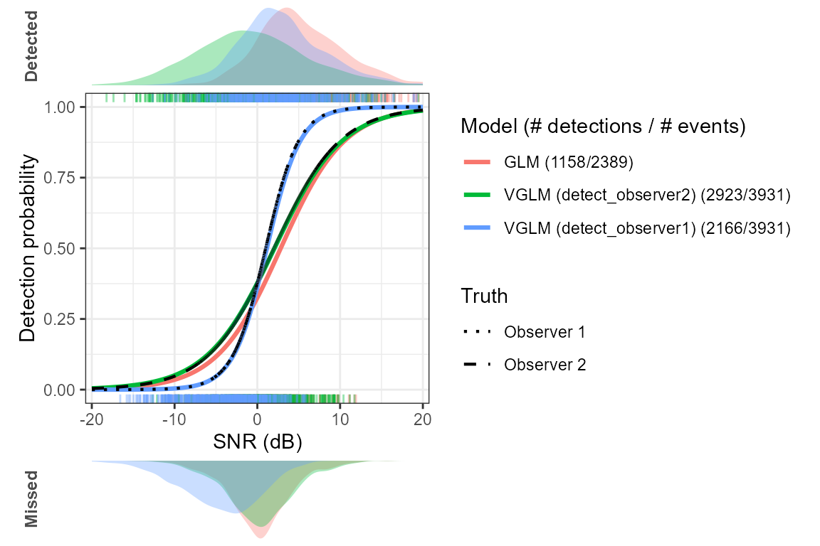
The estimate of Dc derived from the vglm model is very close to the true value for this simulation.
Adjudicated capture-recapture along with independently estimated NL yields more accurate estimates of c and P_a.
Inspect detection functions for insights
# Clone vglm and swap whichObserver for second observer curve
snrDetFun.vglm2 <- snrDetFun.vglm
other_observer  <- setdiff(
  colnames(VGAM::predict(snrDetFun.vglm, newdata = data.frame(SNR = 0),
                         type = "response")),
  snrDetFun.vglm@extra$whichObserver
)[1]
snrDetFun.vglm2@extra$whichObserver <- other_observer

# Ground truth from simulation
truth <- data.frame(
  SNR   = c(simDet2$snr,      capHistTab$snr_observer1),
  p_det = c(simDet2$p_det,    capHistTab$p_det_observer1),
  group = c(rep("Observer 2", nrow(simDet2)),
            rep("Observer 1", nrow(capHistTab)))
)

models <- list(
  "GLM"          = snrDetFun.glm,
  "VGLM obs1"    = snrDetFun.vglm,
  "VGLM obs2"    = snrDetFun.vglm2
)
names(models)[2] <- paste0("VGLM (", snrDetFun.vglm@extra$whichObserver, ")")
names(models)[3] <- paste0("VGLM (", other_observer, ")")

p <- showDetFun(models, distribution = 'density', rug = TRUE, xlim = c(-20, 20))

p <- p +
  ggplot2::geom_line(data = truth, alpha = 1, inherit.aes = FALSE, linewidth = .75,
                     ggplot2::aes(x = SNR, y = p_det, linetype = group)) +
  scale_linetype_manual(values = c("Observer 2" = "dashed",
                                   "Observer 1" = "dotted")) +
  ggplot2::theme(legend.position = "right") +
  labs(color = "Model", linetype = "Truth")

p