Using all available information: a union call density estimate
Source:vignettes/callDensity_unionDetectors.Rmd
callDensity_unionDetectors.Rmd
library(callDensity)
library(VGAM)
#> Loading required package: stats4
#> Loading required package: splines
library(dplyr)
#>
#> Attaching package: 'dplyr'
#> The following objects are masked from 'package:stats':
#>
#>     filter, lag
#> The following objects are masked from 'package:base':
#>
#>     intersect, setdiff, setequal, union
library(ggplot2)
library(kableExtra)
#>
#> Attaching package: 'kableExtra'
#> The following object is masked from 'package:dplyr':
#>
#>     group_rows

# The cde() and pDetInArea() calls are the expensive part of this vignette.
# Their results are cached so that editing prose does not cost hours. The
# simulations themselves are NOT cached: sim is ~100 MB at n = 1e6 and
# rebuilds in minutes, so caching it would put a gigabyte in the repo for
# little gain. From cache this knits in roughly ten minutes.
#
# The cache is only valid for the code that produced it. If you change a
# detector parameter, a sample size, or an outerloop setting, set
# recompute <- TRUE or the tables below will silently show stale numbers.
recompute <- FALSE
cacheDir  <- "precomputed"
if (!dir.exists(cacheDir)) dir.create(cacheDir)

cacheOrRun <- function(name, expr) {
  f <- file.path(cacheDir, paste0(name, ".rds"))
  if (!recompute && file.exists(f)) return(readRDS(f))
  val <- force(expr)
  saveRDS(val, f)
  val
}
Left on the table
Miller et al. (2026) introduced adjudicated capture-recapture (CR) as a way to characterise detectors without assuming any one observer is ground truth, and argued that the method “readily accommodates all available information from multiple observers and/or detectors, if more than one of either is available.” What the paper actually demonstrated, though, was CR producing a call density estimate for each detector, CR1S, CR2S, CRAS and so on in its own terminology, never a single estimate that draws on more than one detector’s own detections at once. The claim about using all available information was true of the underlying capture-recapture model, which is exactly what lets it estimate a false discovery rate without a trusted observer in the first place, but the density estimates built on top of it stayed one-detector-at-a-time throughout.
This vignette closes that gap directly. The capture-recapture model
already estimates, as a normal step in fitting it, the probability that
at least one of several detectors would catch a given call.
This is a standard quantity in double-observer distance sampling, and
callDensity’s own vglmDetectionProb() already computes it
internally as an intermediate step toward each individual detector’s own
detection probability. Surfacing it directly, rather than discarding it,
gives a union detection function: fit one capture-recapture model
jointly on two or more detectors, and read off not just “detector 1’s
own probability of detecting a call” or “detector 2’s own probability,”
but “the probability that detector 1 or detector 2 detects it.”
Paired with the union of their own raw detection counts, how many calls
did either detector flag across the full dataset, this gives a
call density estimate that uses both detectors’ information at once,
rather than two separate, redundant analyses of the same underlying
calls.
The simulation below follows the same setup as
vignette("callDensity_CommonGround"): the same call
population size, the same two detectors, the same adjudicated-subsample
workflow, so the two vignettes can be read side by side. What is new
here is entirely in how the existing per-detector pieces
(Nc, false discovery rate, detection probability) get
combined into one union estimate, not in how any of them are
individually derived.
Simulate a shared call population and two detectors
The call population, source level, noise level, and transmission loss
are exactly as in callDensity_CommonGround: a uniform
distribution of calls in space and time, with acoustic properties
following the passive sonar equation.
n <- 1e6        # number of simulated calls, whether detected or not
R <- 1e6        # radius in m
k <- 1          # number of sensors
minDate <- as.POSIXct("2025-01-01")
maxDate <- as.POSIXct("2026-01-01")
Time <- as.numeric(difftime(maxDate, minDate, unit = "days")) / 365

A <- studyArea(R / 1e3)
TrueCallDensity <- n / (A * Time)

set.seed(1)
sim <- simCallLocation(n = n, R = R, minDate = minDate, maxDate = maxDate)

SL <- data.frame(mean = 190, sd = 4, sampleSize = 350)
NL <- data.frame(mean = 84, sd = 4, sampleSize = n)
tlFunc <- function(r) 20 * log10(r)
sim <- simCallAcoustics(sim, SL, NL, TL = tlFunc)

TL <- simTLradials_20logR(maxRange = R, rangeStep = 1000, numTransects = 8)

cat("Study area (km^2):", A, "\n")
#> Study area (km^2): 3141593
cat("True call density (calls / km^2 / year):", TrueCallDensity, "\n")
#> True call density (calls / km^2 / year): 0.3183099
Two detectors, with the same parameters as
callDensity_CommonGround. Detector 1 is the more sensitive,
more reliable of the two, with a lower threshold and lower false
discovery rate. Detector 2 is noisier on both counts.
det1params <- data.frame(location = 1, scale = 2, func = 'plogis',
                         c = 0.1, fpMean = 0, fpSD = 2)
det2params <- data.frame(location = 2, scale = 4, func = 'plogis',
                         c = 0.3, fpMean = 0, fpSD = 2)

simDet1 <- simulateDetector(det1params, sim)
simDet2 <- simulateDetector(det2params, sim)
Two capture history tables: full year, and adjudicated subsample
Two different tables are needed here, matching a distinction that
already exists for a single detector. Nc always comes from
the full dataset, while the capture history table used to fit a
detection function and estimate a false discovery rate comes from a
small adjudicated subsample. The union case needs both, in the same
shapes as before: a full-year table across both detectors for the union
Nc, and an adjudicated subsample across both detectors for
the joint capture-recapture fit.
Both come from a single merge. The detectors are merged once into a
full-year capture history table, and the subsample is then taken from
that table. This ordering matters. cde() consumes capture
history tables, so the table is the natural object to subsample, and
taking the subsample from the merged table makes it a provable subset of
the full-year table rather than a separately constructed object that
happens to look similar.
# Full year, both detectors. This is what the union Nc comes from. Both
# detectors examined the exact same simulated year, so unionDetections()'s
# fullCoverageConfirmed requirement is satisfied here by construction (see
# ?unionDetections for why this can't be verified automatically from the
# table alone, and has to be confirmed explicitly instead).
capHistTabFull <- simsTocaptureHistoryTable(simDet1, simDet2)

observerCols <- c("detect_observer1", "detect_observer2")

Nc1     <- sum(simDet1$detect_table)
Nc2     <- sum(simDet2$detect_table)
NcUnion <- unionDetections(capHistTabFull, observerCols, fullCoverageConfirmed = TRUE)

cat("Nc, detector 1 alone: ", Nc1, "\n")
#> Nc, detector 1 alone:  101654
cat("Nc, detector 2 alone: ", Nc2, "\n")
#> Nc, detector 2 alone:  173205
cat("Nc, union of both:    ", NcUnion,
    " (between max(Nc1,Nc2) and Nc1+Nc2, as it must be)\n")
#> Nc, union of both:     225744  (between max(Nc1,Nc2) and Nc1+Nc2, as it must be)
# Adjudicated subsample, taken from the merged table. Matches
# callDensity_CommonGround's own 1-hour-in-41 subsampling. subsampleSimInTime()
# defaults to timeCol = 't0', matchbox's own time column, which
# simsTocaptureHistoryTable() writes as a MATLAB datenum.
capHistTab <- subsampleSimInTime(capHistTabFull, interval = "41 hour")

# cde()'s own false-discovery-rate handling needs a single consolidated SNR
# column. This is a separate mechanism from chtToSNRinfo()'s signalCol/noiseCol
# averaging used below.
capHistTab$SNR <- rowMeans(capHistTab[, c("snr_observer1", "snr_observer2")], na.rm = TRUE)

adjudicated <- subset(capHistTab, capHistTab$groundTruth &
                        (capHistTab$detect_observer1 | capHistTab$detect_observer2))

cat("Subsample:", nrow(capHistTab), "events,",
    sum(capHistTab$groundTruth), "of them real calls\n")
#> Subsample: 25815 events, 24352 of them real calls
cat("Adjudicated subsample:", nrow(adjudicated), "true-positive events\n")
#> Adjudicated subsample: 3931 true-positive events
The adjudicated count is worth reporting explicitly, and worth checking. It is the sample that both the detection function and the false discovery rate are estimated from, so it sets the precision of everything downstream. It also cannot exceed the number of real calls in the subsample. If it ever does, something upstream has duplicated events.
One joint model, three ways to read it
Fitting a capture-recapture model with both detectors’ columns as the
two occasions estimates their detection probabilities jointly. This part
does not change at all from a normal two-detector CR analysis. What is
new is asking for three different things back from the same fit, via
whichObserver: detector 1’s own probability, detector 2’s
own probability, and "any" for the probability that at
least one of them detects the call.
fitObs1  <- fitDetFun(adjudicated, modelType = "vglm", yColNames = observerCols,
                      whichObserver = "detect_observer1")
fitObs2  <- fitDetFun(adjudicated, modelType = "vglm", yColNames = observerCols,
                      whichObserver = "detect_observer2")
fitUnion <- fitDetFun(adjudicated, modelType = "vglm", yColNames = observerCols,
                      whichObserver = "any")
VGAM will often emit convergence warnings on a fit like
this, particularly with many occasions. Most are benign.
checkDetFun() reports the things that actually indicate
trouble: the condition number of the covariance matrix, the spread of
the standard errors, and the largest coefficient. This matters because
pDetInArea() propagates detection function uncertainty by
drawing coefficients from that covariance matrix, so an unreliable one
would make the reported CV.pa unreliable too.
checkDetFun(fitUnion)
#> Detection function diagnostics
#>   model type          vglm
#>   coefficients        4
#>   vcov condition no.  108.4
#>   SE range            0.0123 to 0.058 (1.61x median)
#>   largest |coef|      0.5624
#>   IRLS iterations     6
#>   verdict             no problems detected
models <- list("Detector 1" = fitObs1, "Detector 2" = fitObs2, "Union (either)" = fitUnion)

# distribution="none": a union model's own "missed" set is empty by
# construction here (adjudicated is already filtered to events flagged by
# at least one detector, so nothing is left to be "missed by the union"),
# which the density panels below have no data for. The three curves
# themselves make the point without needing that panel.
showDetFun(models, distribution = "none", rug = FALSE)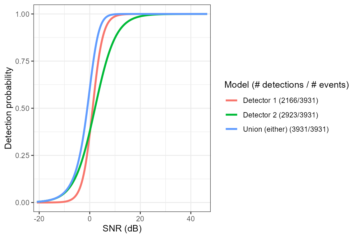
The union curve sits above both individual curves at every SNR, as it must. The probability that either detector catches a call can never be lower than either detector’s own probability on its own.
How many Monte Carlo draws
cde() and pDetInArea() take an
outerloop argument, the number of Monte Carlo draws over
the source level distribution, the noise level distribution, and the
fitted detection function’s coefficients. The package default is 1000.
That is more than this analysis needs, and it is worth being explicit
about why, because outerloop is the single largest lever on
how long anything in this vignette takes to run.
Three quantities converge at different rates. The point estimate
pa is stable by outerloop = 5; running more
draws does not move it. The expected value of CV.pa is also
stable by outerloop = 5. What keeps improving is the
precision of CV.pa: how much the reported CV moves
between repeated Monte Carlo runs on the same fitted model. That
run-to-run spread is about 20% of the CV itself at
outerloop = 5, and about 2% at
outerloop = 250, with no measurable further gain at
1000.
So outerloop = 250 is used below wherever a CV is
reported, and outerloop = 100 in the replicate study, where
the reported CV is averaged over replicates anyway and the residual
Monte Carlo noise averages out.
outerloopReported  <- 250   # anything whose CV goes in a table
outerloopReplicate <- 100   # replicate study, where CVs get averaged
Three call density estimates
cde() itself needs no new arguments for any of this
beyond what already exists. observerCol becomes the vector
c("detect_observer1", "detect_observer2") for the union
case, matching the same detectors the model was fit with
whichObserver = "any" for. cde() checks that
these two agree and refuses to silently combine a union false discovery
rate with a single detector’s own detection probability, or the reverse.
NL is left for cde() to estimate internally
via nlFromDetections(), exactly as it would for a single
detector. No special handling is needed for the union case.
resPair <- cacheOrRun("resPair", list(
  res1 = cde(Nc = Nc1, capHistTab = capHistTab, snrDetFun = fitObs1,
             SL = SL, TL = TL, A = A, T = Time, k = k,
             outerloop = outerloopReported, output.resolution.m = 1000,
             groundTruthCol = "groundTruth", observerCol = "detect_observer1",
             signalCol = c("signalRMSdB_observer1", "signalRMSdB_observer2"),
             noiseCol  = c("noiseRMSdB_observer1",  "noiseRMSdB_observer2")),
  res2 = cde(Nc = Nc2, capHistTab = capHistTab, snrDetFun = fitObs2,
             SL = SL, TL = TL, A = A, T = Time, k = k,
             outerloop = outerloopReported, output.resolution.m = 1000,
             groundTruthCol = "groundTruth", observerCol = "detect_observer2",
             signalCol = c("signalRMSdB_observer1", "signalRMSdB_observer2"),
             noiseCol  = c("noiseRMSdB_observer1",  "noiseRMSdB_observer2"))))

res1 <- resPair$res1
res2 <- resPair$res2
resUnion <- cacheOrRun("resUnion",
  cde(Nc = NcUnion, capHistTab = capHistTab, snrDetFun = fitUnion,
      SL = SL, TL = TL, A = A, T = Time, k = k,
      outerloop = outerloopReported, output.resolution.m = 1000,
      groundTruthCol = "groundTruth", observerCol = observerCols,
      signalCol = c("signalRMSdB_observer1", "signalRMSdB_observer2"),
      noiseCol  = c("noiseRMSdB_observer1",  "noiseRMSdB_observer2")))
Results
resultsTrue <- data.frame(model = "Truth", Nc = n, c = NA, pa = NA,
                          Dc = TrueCallDensity, CV.Dc = 0)

results <- rbind(
  resultsTrue,
  data.frame(model = "Detector 1 alone", Nc = Nc1, c = res1$c, pa = res1$pa,
            Dc = res1$Dc, CV.Dc = res1$CV.Dc),
  data.frame(model = "Detector 2 alone", Nc = Nc2, c = res2$c, pa = res2$pa,
            Dc = res2$Dc, CV.Dc = res2$CV.Dc),
  data.frame(model = "Union (both)", Nc = NcUnion, c = resUnion$c, pa = resUnion$pa,
            Dc = resUnion$Dc, CV.Dc = resUnion$CV.Dc)
)
results$DcFraction <- results$Dc / TrueCallDensity

kableExtra::kbl(results, digits = c(NA, 0, 3, 4, 4, 3, 2), row.names = FALSE,
                col.names = c("Model", "$N_c$", "$\\hat{c}$", "$\\hat{p}_a$",
                             "$D_c$", "$CV.D_c$", "$D_c$ / true $D_c$")) %>%
kableExtra::kable_classic(full_width = FALSE)| Model | / true | |||||
|---|---|---|---|---|---|---|
| Truth | 1000000 | NA | NA | 0.3183 | 0.000 | 1.00 |
| Detector 1 alone | 101654 | 0.093 | 0.0918 | 0.3195 | 0.096 | 1.00 |
| Detector 2 alone | 173205 | 0.298 | 0.1272 | 0.3043 | 0.078 | 0.96 |
| Union (both) | 225744 | 0.271 | 0.1715 | 0.3053 | 0.073 | 0.96 |
plotData <- subset(results, model != "Truth")
plotData$model <- factor(plotData$model, levels = plotData$model)

ggplot2::ggplot(plotData, ggplot2::aes(x = model, y = Dc, fill = model)) +
  ggplot2::geom_col(width = 0.6) +
  ggplot2::geom_errorbar(ggplot2::aes(ymin = Dc * (1 - CV.Dc), ymax = Dc * (1 + CV.Dc)),
                        width = 0.15) +
  ggplot2::geom_hline(yintercept = TrueCallDensity, linetype = "dashed", colour = "grey30") +
  ggplot2::annotate("text", x = 0.6, y = TrueCallDensity, label = "Truth",
                    vjust = -0.5, hjust = 0, colour = "grey30", size = 3) +
  ggplot2::labs(x = NULL, y = expression(D[c]~(calls~km^-2~year^-1)), fill = NULL) +
  ggplot2::theme_bw() +
  ggplot2::theme(legend.position = "none")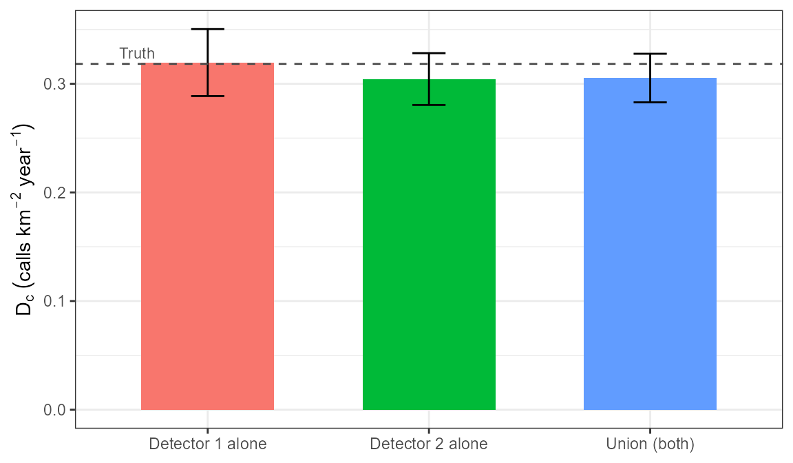
When this helps, and when it might not
The false discovery rate’s own coefficient of variation is smaller for the union than for either individual detector, always. It only depends on how many adjudicated events went into estimating it, and the union pools strictly more of them, every event either detector flagged, than either detector’s own count alone does. That part of the improvement is guaranteed by construction, not a property of this particular simulation.
The detection probability’s own uncertainty is a different matter, and it is the one that actually decides whether the union wins overall. The union curve is a genuinely new quantity, not simply a better-sampled version of either individual curve, and its own precision depends on how well the joint model’s coefficients happen to be estimated in a given dataset. That is not guaranteed to be tighter than an individual detector’s own curve when that detector is already well characterised on its own.
So the honest summary is that the union’s false discovery rate is unconditionally tighter, and the union is never worse than the worse of the two detectors here, but it is not a guarantee of beating the better one. That comes down to how well that detector’s own curve happens to be identified in a given dataset, a separate question from the union’s own construction. The replicate study below quantifies how often each outcome occurs rather than leaving it as an assertion.
What the union approach always buys, regardless of how that particular contest goes, is using detections that a single-detector analysis discards outright. A call caught only by detector 2 contributes nothing to a “detector 1 alone” estimate’s own count, adjudicated sample, or detection function, even though it is exactly the kind of information adjudicated capture-recapture was introduced to make use of.
Scaling to more detectors
Automated detectors are becoming a commodity for some species and call types. Running ten mediocre detectors costs little more than running two, unlike the human observer effort adjudicated capture-recapture was originally built around. If that is the actual situation, the two-detector case above is really a lower bound on what is available. This section repeats the same union analysis for 2 to 10 detectors of varying quality, sharing the same underlying call population, to see how the false discovery rate’s guaranteed improvement plays out as the pool grows.
Ten detectors, with threshold, steepness, and false discovery rate all drawn randomly from a plausible “commodity” range inspired by prior estimates (e.g. Miller et al. (2026)’s own observed detectors), rather than assigned as a deliberate sequence. A fixed, ordered progression of qualities across detector count risks tying “more detectors” to “detectors added later happen to be better or worse,” which is a property of the specific sequence chosen, not of pooling more detectors. Random, independent draws avoid that. The 2 to 10-detector comparisons use the first 2, first 4, and so on up to all 10 of the same drawn pool, so adding detectors here means literally adding to the same set rather than swapping in a different one.
nMax <- 10
set.seed(42)
locations <- rnorm(nMax, mean = 2.5, sd = 1)
scales    <- pmax(rnorm(nMax, mean = 3, sd = 1), 0.5)  # guard against a nonsensical near-zero scale
fdrs      <- runif(nMax, 0.1, 0.4)

detParamsN <- lapply(seq_len(nMax), function(i) {
  data.frame(location = locations[i], scale = scales[i], func = 'plogis',
            c = fdrs[i], fpMean = 0, fpSD = 2)
})

simDetsN <- lapply(seq_len(nMax), function(i) simulateDetector(detParamsN[[i]], sim))
runUnionAnalysis <- function(N) {
  detsSubset <- simDetsN[1:N]

  # Merge once, then subsample the merged table.
  capHistTabFullN <- do.call(simsTocaptureHistoryTable, detsSubset)
  capHistTabN     <- subsampleSimInTime(capHistTabFullN, interval = "41 hour")
  capHistTabN$SNR <- rowMeans(capHistTabN[, paste0("snr_observer", seq_len(N))], na.rm = TRUE)

  observerColsN <- paste0("detect_observer", seq_len(N))
  signalColsN   <- paste0("signalRMSdB_observer", seq_len(N))
  noiseColsN    <- paste0("noiseRMSdB_observer", seq_len(N))

  NcUnionN <- unionDetections(capHistTabFullN, observerColsN, fullCoverageConfirmed = TRUE)

  adjudicatedN <- subset(capHistTabN, capHistTabN$groundTruth &
                           Reduce(`|`, as.list(capHistTabN[observerColsN])))

  fitUnionN <- fitDetFun(adjudicatedN, modelType = "vglm", yColNames = observerColsN,
                         whichObserver = "any")

  resUnionN <- cde(Nc = NcUnionN, capHistTab = capHistTabN, snrDetFun = fitUnionN,
                   SL = SL, TL = TL, A = A, T = Time, k = k,
                   outerloop = outerloopReported, output.resolution.m = 1000,
                   groundTruthCol = "groundTruth", observerCol = observerColsN,
                   signalCol = signalColsN, noiseCol = noiseColsN)

  data.frame(N = N, nAdj = nrow(adjudicatedN), Nc = NcUnionN,
            c = resUnionN$c, pa = resUnionN$pa,
            Dc = resUnionN$Dc, CV.Dc = resUnionN$CV.Dc,
            DcFraction = resUnionN$Dc / TrueCallDensity)
}


scalingResults <- cacheOrRun("scalingResults",
  do.call(rbind, lapply(c(2, 4, 6, 8, 10), runUnionAnalysis)))

kableExtra::kbl(scalingResults, digits = c(0, 0, 0, 3, 4, 4, 3, 2), row.names = FALSE,
                col.names = c("N detectors", "adjudicated $n$", "$N_c$",
                             "$\\hat{c}$", "$\\hat{p}_a$",
                             "$D_c$", "$CV.D_c$", "$D_c$ / true $D_c$")) %>%
kableExtra::kable_classic(full_width = FALSE)| N detectors | adjudicated | / true | |||||
|---|---|---|---|---|---|---|---|
| 2 | 5230 | 285907 | 0.253 | 0.2106 | 0.3230 | 0.061 | 1.01 |
| 4 | 5945 | 369537 | 0.342 | 0.2480 | 0.3121 | 0.050 | 0.98 |
| 6 | 7144 | 508478 | 0.426 | 0.2957 | 0.3140 | 0.045 | 0.99 |
| 8 | 7340 | 573632 | 0.477 | 0.3195 | 0.2990 | 0.040 | 0.94 |
| 10 | 8246 | 681019 | 0.502 | 0.3550 | 0.3042 | 0.039 | 0.96 |
The adjudicated sample size is in the table because it is what the false discovery rate’s precision depends on directly, and because it is the quantity to check first if anything looks wrong. It rises with detector count, since each additional detector adds events that no earlier detector flagged, but it can never exceed the number of real calls in the subsample.
ggplot2::ggplot(scalingResults, ggplot2::aes(x = N, y = CV.Dc)) +
  ggplot2::geom_line() +
  ggplot2::geom_point(size = 2) +
  ggplot2::scale_x_continuous(breaks = scalingResults$N) +
  ggplot2::labs(x = "Number of detectors in the union", y = expression(CV.D[c])) +
  ggplot2::theme_bw()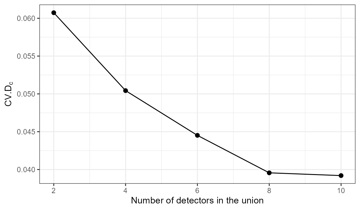
SNR and detector agreement
Miller et al. (2026)’s Figure 3 showed
the SNR distribution of adjudicated detections split by how many
observers or detectors agreed on them, with true and false positives
plotted as mirrored half-violins at each agreement count. The
false-positive half is not reproduced here. In this simulation, each
detector’s own false positives are independently, randomly timed, so two
of them coinciding is impossible by construction:
simulateDetector() draws false positive times that are
guaranteed distinct from every real call time and from each other. An
event two or more simulated detectors agree on is therefore always a
real call here, which would make any true-versus-false comparison at
higher agreement counts an artifact of the simulation rather than a real
finding. That is a simulation limitation already on record as a to-do in
callDensity_CommonGround, and it needs a proper mechanism
for correlating false positives across detectors before the
false-positive half can be revisited.
The true-positive half does not have that problem, since it says nothing about false positives at all. It shows only whether genuine calls caught by more detectors tend to sit at higher SNR, which is true by the ordinary logic of every detector improving with SNR, independent of how any detector’s false positives happen to be simulated.
detsSubset10 <- simDetsN[1:10]
chFull10     <- do.call(simsTocaptureHistoryTable, detsSubset10)
capHistTab10 <- subsampleSimInTime(chFull10, interval = "41 hour")
capHistTab10$SNR <- rowMeans(capHistTab10[, paste0("snr_observer", 1:10)], na.rm = TRUE)
observerCols10 <- paste0("detect_observer", 1:10)

adjudicatedPositive <- subset(capHistTab10, capHistTab10$groundTruth &
                                Reduce(`|`, as.list(capHistTab10[observerCols10])))
adjudicatedPositive$nAgree <- rowSums(adjudicatedPositive[, observerCols10])

ggplot2::ggplot(adjudicatedPositive, ggplot2::aes(x = factor(nAgree), y = SNR)) +
  ggplot2::geom_violin(fill = "steelblue", alpha = 0.6, scale='count', width=3) +
  ggplot2::labs(x = "Number of detectors agreeing", y = "SNR (dB)") +
  ggplot2::theme_bw()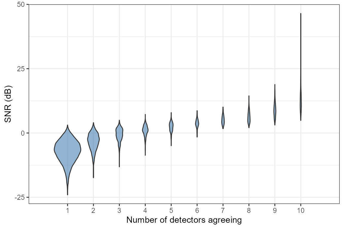
Higher-SNR calls are the ones every detector in the pool is more likely to catch, so as more detectors agree, the SNR distribution shifts up and narrows. Calls at the far right, caught by all ten, sit well clear of the noise floor. Calls caught by only one sit close to it, exactly the population where any individual detector’s own threshold is doing the most work.
Is the trend in real?
The scaling plot above reports one per detector count. A single draw per point cannot support any claim about the ordering between points, and it is worth being blunt about that rather than reading a trend off it. To find out whether the ordering means anything, the whole analysis has to be repeated on fresh simulated data.
Repeating it also allows a second, more useful comparison. Each replicate reports its own , an estimate of how much would vary if the analysis were repeated. Across replicates the actual variation in can be measured directly. The two should agree. Whether they do is a check on the variance machinery that no single analysis can perform on itself.
runReplicate <- function(simSeed, N) {
  nRep <- 1e6
  set.seed(simSeed)
  simR <- simCallLocation(n = nRep, R = R, minDate = minDate, maxDate = maxDate)
  NLrep <- data.frame(mean = 84, sd = 4, sampleSize = nRep)
  simR <- simCallAcoustics(simR, SL, NLrep, TL = tlFunc)
  trueDcRep <- nRep / (A * Time)

  detsR <- lapply(seq_len(N), function(i) simulateDetector(detParamsN[[i]], simR))

  # Merge once, then subsample the merged table.
  chFullR <- do.call(simsTocaptureHistoryTable, detsR)
  chR     <- subsampleSimInTime(chFullR, interval = "41 hour")
  chR$SNR <- rowMeans(chR[, paste0("snr_observer", seq_len(N))], na.rm = TRUE)

  ocR <- paste0("detect_observer", seq_len(N))
  NcR <- unionDetections(chFullR, ocR, fullCoverageConfirmed = TRUE)
  adjR <- subset(chR, chR$groundTruth & Reduce(`|`, as.list(chR[ocR])))
  fitR <- fitDetFun(adjR, modelType = "vglm", yColNames = ocR, whichObserver = "any")

  resR <- cde(Nc = NcR, capHistTab = chR, snrDetFun = fitR,
              SL = SL, TL = TL, A = A, T = Time, k = k,
              outerloop = outerloopReplicate, output.resolution.m = 1000,
              groundTruthCol = "groundTruth", observerCol = ocR,
              signalCol = paste0("signalRMSdB_observer", seq_len(N)),
              noiseCol  = paste0("noiseRMSdB_observer", seq_len(N)))

  data.frame(N = N, seed = simSeed, nAdj = nrow(adjR),
             Dc = resR$Dc, trueDc = trueDcRep,
             DcRatio = resR$Dc / trueDcRep, reportedCV = resR$CV.Dc)
}

nSeeds <- 10

replicateRuns <- cacheOrRun("replicateRuns", {
  replicateGrid <- expand.grid(seed = seq_len(nSeeds), N = c(2, 6, 10))
  do.call(rbind, Map(runReplicate, replicateGrid$seed, replicateGrid$N))
})
replicateSummary <- replicateRuns %>%
  dplyr::group_by(N) %>%
  dplyr::summarise(
    nAdj         = round(mean(nAdj)),
    meanDcRatio  = mean(DcRatio),
    realizedCV   = sd(Dc) / mean(Dc),
    reportedCV   = mean(reportedCV),
    ratio        = realizedCV / reportedCV,
    .groups = "drop"
  )

kableExtra::kbl(replicateSummary, digits = 3, row.names = FALSE,
                col.names = c("N detectors", "adjudicated $n$",
                             "mean $D_c$ / true $D_c$",
                             "realized CV", "mean reported $CV.D_c$",
                             "realized / reported")) %>%
kableExtra::kable_classic(full_width = FALSE)| N detectors | adjudicated | mean / true | realized CV | mean reported | realized / reported |
|---|---|---|---|---|---|
| 2 | 5228 | 0.992 | 0.058 | 0.060 | 0.961 |
| 6 | 7157 | 0.987 | 0.027 | 0.043 | 0.636 |
| 10 | 8266 | 0.976 | 0.022 | 0.039 | 0.558 |
The last column is the check. If the variance machinery is working it should sit near 1. Values below 1 mean the reported CV is conservative, overstating how much the estimate actually moves. Values above 1 are the dangerous direction, false confidence.
It carries real sampling error, though, and that has to be stated rather than glossed over. A standard deviation computed from 10 replicates has a sampling error of roughly 24%, and a ratio of two such quantities carries more. No single row of this table is on its own distinguishable from 1. What makes the pattern worth reading is that the ratio falls consistently as detectors are added, which is a trend across rows rather than three independent noisy draws.
The mean / true column deserves the same attention as the CV columns, and points the other way. It sits slightly below 1 throughout, and drifts a little further below as detectors are added. The estimator is close to unbiased, but not exactly, and the small negative bias grows with the same thing the conservative CV is a property of. The two partly cancel: a wide interval that is slightly off-centre covers the truth about as often as a correctly sized one that is centred, which is why the coverage below lands near nominal rather than above it despite the conservative CV.
A more directly useful question is whether a confidence interval built from the reported CV actually contains the truth. That has an unambiguous target: a nominal 95% interval should contain it 95% of the time.
z <- qnorm(0.975)
coverage <- replicateRuns %>%
  dplyr::mutate(seLog = sqrt(log(1 + reportedCV^2)),   # Buckland lognormal CI
                lo    = Dc * exp(-z * seLog),
                hi    = Dc * exp( z * seLog)) %>%
  dplyr::group_by(N) %>%
  dplyr::summarise(nRep     = dplyr::n(),
                   coverage = mean(trueDc >= lo & trueDc <= hi),
                   meanRelWidth = mean((hi - lo) / Dc),
                   .groups = "drop")

kableExtra::kbl(coverage, digits = 3, row.names = FALSE,
                col.names = c("N detectors", "replicates",
                             "95% CI coverage", "mean relative CI width")) %>%
kableExtra::kable_classic(full_width = FALSE)| N detectors | replicates | 95% CI coverage | mean relative CI width |
|---|---|---|---|
| 2 | 10 | 1.0 | 0.236 |
| 6 | 10 | 0.9 | 0.168 |
| 10 | 10 | 0.9 | 0.152 |
The lognormal interval is used here because it is the distance sampling convention and because it cannot go negative at large CV. With 10 replicates, coverage is measurable to roughly ten percentage points, which is enough to distinguish 0.7 from 0.95 but not 0.9 from 0.95.
Reporting uncertainty honestly
cde()’s
combines three components in quadrature: the CV of
,
of
,
and of
.
Four things about that combination are worth knowing before quoting the
result.
is treated as exact. cde() sets its CV to zero.
The package provides Nc_CV(), which computes the binomial
expression instead, and the two differ. The zero is harmless when
is large, since the binomial CV is roughly
,
which is well under a percent for a year of detections and disappears
under quadrature against a
of a few percent. It is not harmless for a short deployment or a rare
call type. The check is one line, and it is worth doing rather than
assuming.
The components are assumed independent. and come from the same adjudicated table and, in the union case, from the same joint model, so their errors need not be independent. Because depends on in the numerator and in the denominator, a negative correlation between them makes quadrature conservative and a positive one makes it optimistic. Which way it goes is a property of the data, not something to assume.
The noise level’s effective sample size is not the number of
detections. nlFromDetections() returns
sampleSize equal to the number of detections it estimated
from, which is correct here because this simulation draws noise
independently for every call. Real ambient noise is autocorrelated over
hours and real detections cluster in time, so the number of genuinely
independent noise measurements is far smaller than the number of
detections. Passing the detection count instead will understate the
noise level’s contribution to
.
is conditional on one fitted model. It propagates uncertainty in the coefficients of a single detection function and has no way to see how differently the analysis would have gone with a different set of detectors. The jackknife below gets at that directly.
Detector-set sensitivity on real data
The replicate study above needs something real analyses never have:
the ability to generate fresh datasets. With one dataset and a fixed set
of detectors, jackknifeDetectors() gets at the same
question from the other direction. Refit the union estimate once per
detector, each time leaving that detector out, and see how far the
answer moves.
This is leave-one-out refitting, structurally like leave-one-out cross-validation, but aimed at a different target. Cross-validation estimates prediction error by scoring a model on held-out data, whereas the jackknife estimates an estimator’s own sensitivity by watching how much it moves as each unit is removed. Here the unit removed is a whole detector, so what comes back is detector-set sensitivity.
# chFull10 and capHistTab10 were built above, merged once then subsampled.
jk <- cacheOrRun("jackknife", jackknifeDetectors(
  capHistTab   = capHistTab10,
  observerCols = paste0("detect_observer", 1:10),
  signalCols   = paste0("signalRMSdB_observer", 1:10),
  noiseCols    = paste0("noiseRMSdB_observer", 1:10),
  NcTable      = chFull10, fullCoverageConfirmed = TRUE,
  SL = SL, TL = TL, A = A, T = Time, k = k,
  outerloop = outerloopReplicate, output.resolution.m = 1000))

kableExtra::kbl(jk[, c("dropped", "Dc", "pa", "c", "shift")], digits = 4,
                row.names = FALSE,
                col.names = c("Detector dropped", "$D_c$", "$\\hat{p}_a$",
                             "$\\hat{c}$", "shift in $D_c$")) %>%
kableExtra::kable_classic(full_width = FALSE)| Detector dropped | shift in | |||
|---|---|---|---|---|
| detect_observer1 | 0.2974 | 0.3343 | 0.5027 | -0.0084 |
| detect_observer2 | 0.2885 | 0.3025 | 0.5190 | -0.0173 |
| detect_observer3 | 0.3098 | 0.3470 | 0.4975 | 0.0040 |
| detect_observer4 | 0.3026 | 0.3477 | 0.4717 | -0.0032 |
| detect_observer5 | 0.3062 | 0.3412 | 0.4923 | 0.0004 |
| detect_observer6 | 0.2978 | 0.3370 | 0.4655 | -0.0079 |
| detect_observer7 | 0.3055 | 0.3473 | 0.4789 | -0.0003 |
| detect_observer8 | 0.3135 | 0.3440 | 0.4859 | 0.0077 |
| detect_observer9 | 0.3036 | 0.3550 | 0.4865 | -0.0021 |
| detect_observer10 | 0.3005 | 0.3186 | 0.4946 | -0.0052 |
data.frame(
  quantity = c("cde()'s own reported CV.Dc (full 10-detector fit)",
               "jackknife CV across leave-one-out refits"),
  value = c(attr(jk, "full")$CV.Dc, attr(jk, "jackknifeCV"))
) %>%
  kableExtra::kbl(digits = 4, row.names = FALSE, col.names = c("", "value")) %>%
kableExtra::kable_classic(full_width = FALSE)| value | |
|---|---|
| cde()’s own reported CV.Dc (full 10-detector fit) | 0.0402 |
| jackknife CV across leave-one-out refits | 0.0662 |
The jackknife CV and the reported measure different things, and quoting both is more informative than quoting either alone. The reported CV is conditional on one fitted model and one detector set. The jackknife varies the detector set and can see a source of variation the internal calculation is structurally blind to.
A large shift for one detector is a signal to look, not a verdict. A detector contributing genuinely distinct information should move the estimate when it is removed. That is what contributing means. What the shifts identify is which detectors the answer actually depends on, which is worth knowing before trusting it, and worth reporting alongside it.
A note on where the real uncertainty lives
Detector-set sensitivity is measurable, and the two sections above measure it. It is also, on this evidence, not the leading source of error in a call density estimate. The shifts in the jackknife table are small next to what a mis-specified noise level distribution can do. An error of a few dB in the assumed , well within the range of what a real deployment’s noise characterisation might be off by, moves by considerably more than dropping the most influential detector here does. Transmission loss and source level are, if anything, less well characterised than noise level in most real analyses, and the assumption that calls are uniformly distributed in space is a structural approximation this simulation satisfies exactly and real data never does.
So the honest ordering is to worry about , , and the spatial distribution first, and to treat detector-set composition as a second-order concern worth a cheap diagnostic rather than a redesign. The jackknife costs refits and needs no ground truth, which makes it cheap enough to run anyway.